Introduction
Gaussian processes
GPs are probability distributions over functions and useful non-parametric models for probabilistic regression. A GP is defined as a set of random variables, any finite number of which is jointly Gaussian distributed.
They are fully specified by a mean function $m$ and a covariance function (kernel) $k$, which are used to compute the mean vector and the covariance matrix of the joint distribution of a finite number of random variables.
A function can be considered an infinitely long vector $f_1,f_2,\ldots$ of function values at corresponding input locations $\mathbf x_1,~\mathbf x_2, \ldots$. One of the most straightforward ways to place a distribution on these function values would be a Gaussian distribution. However, the Gaussian distribution is only defined for finite-dimensional vectors and not for functions. The Gaussian process generalizes the Gaussian distribution to this setting by describing any finite subset of (random) function values by a joint Gaussian distribution. This is practically relevant, since we are usually only interested in finite training and test sets. If we partition the set of all function values into training set $\mathbf{f}$, test set $\mathbf{f}_*$ and "other" function values, the marginalization property of the Gaussian allows us to integrate out infinitely many "other" function values to obtain a finite joint Gaussian distribution $p(\mathbf f, \mathbf f_*)$ with mean $\mathbf m$ and covariance matrix $\mathbf K$ given by
respectively. The entries of the mean vector and the covariance matrix can be computed using the mean and covariance functions of the GP, such that $m_i = m(\mathbf x_i)$, $K_{ij} = k(\mathbf x_i,\mathbf x_j),$ where $\mathbf x_i, \mathbf x_j$ are from the training or test sets. Gaussian conditioning on this joint distribution yields the Gaussian predictive distribution of function values $\mathbf f_*$ at test time as
The GP is a useful and flexible model, and good software
Regression setting
We consider a regression problem
where $\mathbf{x}\in\mathbb{R}^D$, $y\in\mathbb{R}$, and $\epsilon\sim \mathcal N(0,\sigma_n^2)$ is i.i.d. Gaussian measurement noise. We place a GP prior on the unknown function $f$, such that the generative process is
where $p(f)$ is the GP prior and $p(y|f, \mathbf{x})$ is the likelihood. Moreover, $m$ and $k$ are the mean and covariance functions of the GP, respectively.
For training inputs $\mathbf X = [\mathbf x_1, \ldots, \mathbf x_N]$ and corresponding (noisy) training targets $\mathbf y = [y_1,\ldots, y_N]$ we obtain the predictive distribution
at a test point $\mathbf{x}_*$.
2.1 Mean and covariance functionsMean and covariance functions
The prior mean function $m(\cdot)$ describes the average function under the GP distribution before seeing any data. Therefore, it offers a straightforward way to incorporate prior knowledge about the function we wish to model. For example, any kind of (idealized) mechanical or physics model can be used as a prior. The GP would then model the discrepancy between this prior and real-world data. In the absence of this type of prior knowledge, a common choice is to set the prior mean function to zero, i.e., $m(\cdot)\equiv 0$. This is the setting we consider in the following. However, everything we will discuss also holds for general prior mean functions.
The covariance function $k(\mathbf{x}, \mathbf{x}^\prime)$ computes the covariance $cov[f(\mathbf{x}), f(\mathbf{x}^\prime)]$ between the corresponding function values by evaluating the covariance function $k$ at the corresponding inputs $\mathbf{x}, \mathbf{x}^\prime$ (kernel trick
Marginal likelihood and GP training
To train the GP, we maximize the marginal likelihood
where $\mathbf K$ is the kernel matrix with $K_{ij}=k(\mathbf x_i, \mathbf x_j)$. $\mathbf X = [\mathbf x_1,\ldots, \mathbf x_N]^T$ are the training inputs, and $\mathbf y = [y_1,\ldots, y_N]^T$ are the corresponding training targets.
The hyperparameters $\mathbf\theta$ appear non-linearly in the kernel matrix $\mathbf{K}$, and a closed-form solution to maximizing the marginal likelihood cannot be found in general. In practice, we use gradient-based optimization algorithms (e.g., conjugate gradients or BFGS) to find a (local) optimum of the marginal likelihood.
Remark.
Maximizing the marginal likelihood behaves much better than finding maximum likelihood or maximum a-posteriori point estimates
Stationary covariance functions and hyperparameters
Hyperparameters play a central role in Gaussian processes, as they control high-level properties of the prior through the mean and covariance functions. The hyperparameters may also cause some practical issues (e.g., numerical instability) during inference. However, the GP often allows for an interpretation of its small number of hyperparameters, which can be used to address those practical issues.
In the following, we will exclusively focus our discussion on stationary covariance functions (kernels) for interpreting these hyperparameters. Stationarity implies that the covariance function only depends on distances $\|\mathbf{x} - \mathbf{x}^\prime\|$ of the corresponding inputs, and not on the location of the individual data points. This means that if the inputs are close to each other, the corresponding function values are strongly correlated. Therefore, stationary covariance functions can also be written as $k(\tau)$, where $\tau = \|\mathbf{x} - \mathbf{x}^\prime\|$.
Commonly used stationary covariance functions are the Gaussian (squared exponential, exponentiated quadratic, RBF) and the Matern family:
The parameters of these covariance functions are the lengthscale $l$ and the signal variance $\sigma_f^2$. The parameters of the covariance function are the hyperparameters of the GP and control the GP distribution.
Interpretation of the hyperparameters
In the following, we will provide insights into what these hyperparameters mean and how they can be interpreted. These insights can not only help us initializing the optimization of the hyperparameters to 'meaningful' values; they also allow us to identify, explain and address some of the problems we encounter when working with Gaussian processes. Throughout the following, we make the assumption that the zero mean and a stationary covariance function make sense.
4.1 LengthscalesLengthscales
1:
The correlation between function values $f(\mathbf{x})$ and $f(\mathbf{x}^\prime)$ depends on the (scaled) distance $\tau/l =\|\mathbf{x} -\mathbf{x}^\prime\|/l$ of the corresponding inputs. Function values are strongly correlated only if the corresponding inputs are close to each other, where "close" depends on the lengthscale parameter $l$.
For this figure we use the Gaussian kernel.

Stationary covariance functions typically contain the term
2:
Samples from a Gaussian process with different lengthscales.
Signal variance
The signal variance parameter $\sigma_f^2$ allows us to say something about the amplitude of the function we model. The covariance function can generally be written as
3:
Samples from a Gaussian process prior (mean function $m\equiv 0$, lengthscale $l=1$) with
different signal variances $\sigma_f^2$.
Noise variance
The noise variance $\sigma_n^2$ is not a direct parameter of the GP, but a parameter of the likelihood function. It indicates how much measurement noise the observations contain. In the basic model we consider in this article, the function values $f(\mathbf{x})$ are corrupted by i.i.d. Gaussian noise with mean $0$ and variance $\sigma_n^2$. If the measurement noise is $0$, the posterior mean function of the GP will pass through all observations. This may require a complex function with many changes in direction. If the measurement noise is big, the posterior mean function will not necessarily pass through the observations. Instead, it smoothes out the noisy observations.
4: Samples from a Gaussian process prior (mean function $m\equiv 0$, lengthscale $l=0.1$, signal variance $\sigma_f^2=1.0$) with different noise variances $\sigma_n^2$.
Figure 4 shows samples from a GP prior with a fixed lengthscale and signal variance but varying noise variance. The greater the noise variance, the noisier the observations (colored) of the underlying sampled function (black, solid). We fixed the random seed to allow for an easier comparison of the noise effect on the GP samples. For greater values of $\sigma_n$, the noise dominates the signal of the underlying function.
5 Hyperparameter optimizationHyperparameter optimization
When training the Gaussian process, the standard procedure is to maximize the marginal likelihood $p(\mathbf{y}|\mathbf{X},\mathbf{\theta})$ with respect to the GP hyperparameters $\mathbf{\theta}$. The marginal likelihood is non-convex with potentially multiple local optima. Therefore, we may end up in (bad) local optima when we choose a gradient-based optimization method (e.g., conjugate gradients or BFGS). This happens more often in the small-data regime, where data can be interpreted in multiple ways. Figure 5 shows an example of the log-marginal likelihood with three different local optima. The figure shows the log-marginal likelihood contour as a function of the lengthscale and noise parameters. For every pair $(l, \sigma_n)$ we found the best signal variance parameter (not displayed).
5: Training data (orange discs), log-marginal likelihood contour and three possible GP fits (left-bottom and right-hand panels) corresponding to the
three local optima at $(\sigma_n, l) = (0.02, 0.36)$, $(0.97, 5.80)$, $(0.76, 1.13)$, respectively. All three hyperparameter settings and, therefore, the corresponding GP
models make sense: While the bottom left GP model explains
the (noisy) data well, the top right GP fit
explains the data by a near-linear function (long lengthscale) and an high noise level.
The global optimum (bottom right) has a slightly better log-marginal likelihood value and is a compromise between the other two other local optima, discovering the latent sinusoidal wave that generated the data while accounting for a fairly high level of measurement noise.
Regions of attraction.
With an increasing size of the training dataset, the marginal likelihood tends to have a single optimum (possibly with huge plateaus).
In the following, we provide some practical guidelines for initializing the hyperparameters, which may be useful to find good local optima.
5.1 Hyperparameter initiatlizationInitialization of the hyperparameters: useful heuristics
Earlier, we interpreted the standard hyperparameters of a GP: the signal variance and the lengthscales for the covariance function, and the noise variance for the (Gaussian) likelihood. In order to initialize these parameters to reasonable values when we optimize the marginal likelihood, we need to align them with what we know about the data, either empirically or using prior knowledge. Assume, we have training inputs $\mathbf{X}$ and training targets $\mathbf{y}$. We will see that the signal and noise variances can be initialized using statistics of the training targets, whereas the lengthscale parameters can be initialized using statistics of the training inputs.
In our standard model, where we assume i.i.d. Gaussian noise and a prior mean function $m\equiv 0$, the variability in the observations $y_i = f(\mathbf{x}_i) + \epsilon,~\epsilon\sim\mathcal N(0,\sigma_n^2)$, has two sources: A structured fluctation due to the function $f$ and a purely random component due to the independent measurement noise. The corresponding contributions to the variance of the observations are given by the signal variance $\sigma_f^2$ and the noise variance $\sigma_n^2$, respectively:
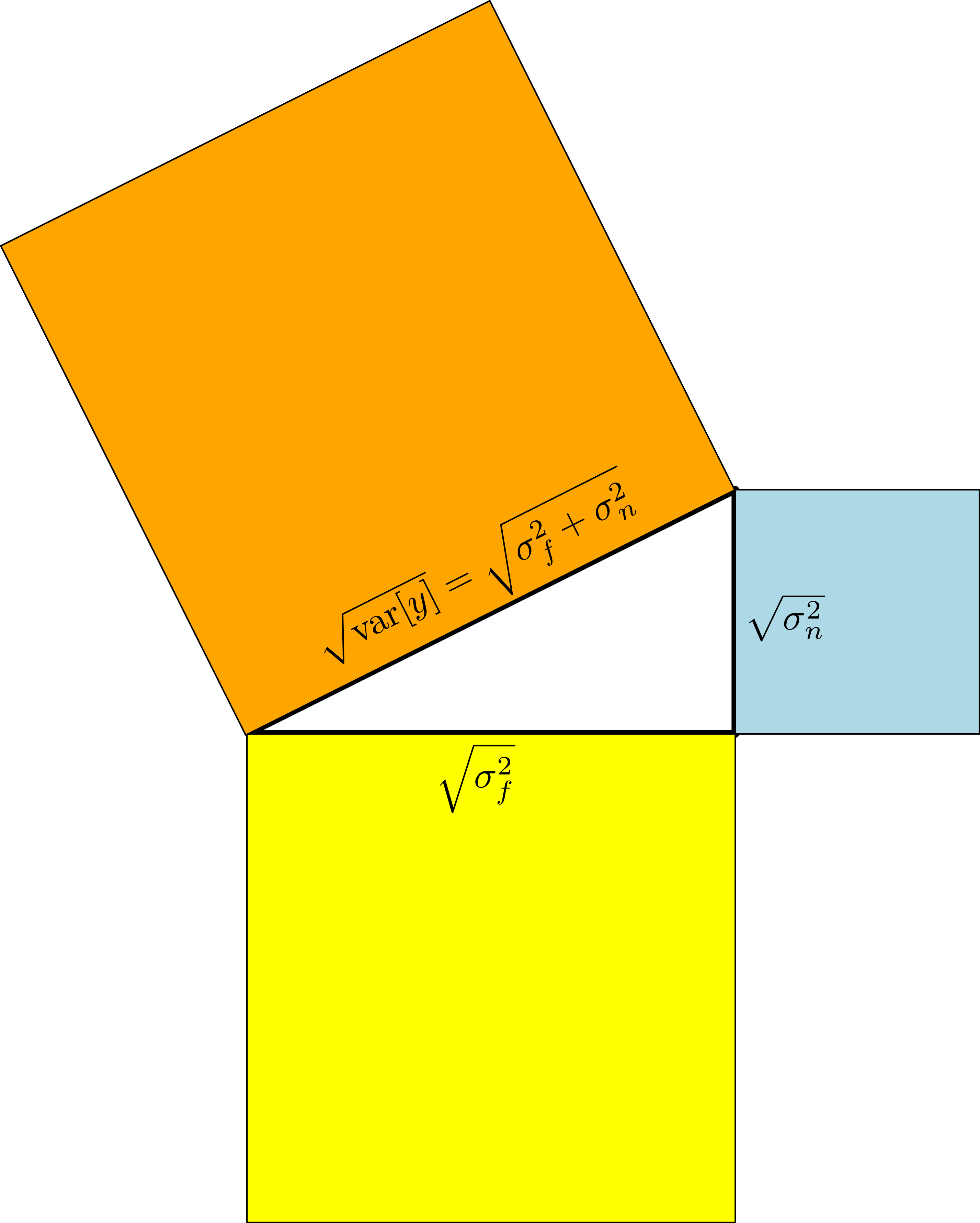
Due to the independence of the signal variance $\sigma_f^2$ and the noise variance $\sigma_n^2$, their corresponding vectors are orthogonal. Using the Pythagoraen theorem, we obtain $\text{var}[y] = \sigma_f^2 + \sigma_n^2$ from a geometric perspective.
Prior knowledge about measurement noise or signal variance.
The noise variance embodies the amount of measurement noise we expect in the observations $\mathbf{y}$. Reasonable (initial) values would be in the range $\big[0, \text{var}[\mathbf y]\big]$. Sometimes, we have some prior knowledge about the measurement noise (e.g., if we use sensors, such as cameras or lasers where we can find these values in the technical specification), we should set the measurement noise to these values, and the signal variance to $\sigma_f^2 \approx \text{var}[\mathbf{y}] - \sigma_n^2$.
6
Initialization for the signal variance.
Sometimes, we know something about the amplitude of the function we wish to model (e.g., if we consider a sinusoidal function ranging between -1 and +1, the amplitude is 2). In these cases, it makes sense to initialize the signal variance, such that $\sqrt{\sigma_f^2}\approx \frac{\text{amplitude}}{2}$ and $\sigma_n^2 = \text{var}[\mathbf{y}] -\sigma_f^2$. Since the function values are jointly Gaussian distributed in a GP, we would expect that the observed function values are reasonably well covered by this variance.
Unknown signal and noise variance If we know nothing specific about the noise variance or the signal variance, we can still make some practical assumptions: From a practical point of view, there is not much use of attempting to model a function where the noise variance is greater than the signal variance (the signal-to-noise ratio would be smaller than 1). Therefore, we should initialize the signal variance to a value greater than the noise variance: $\sigma_f^2 > \sigma_n^2$.
7
Initialization for the unknown signal and noise variance.
In this example, we consider fitting a GP using noise-corrucpted data (gray dots)
from an unknown function f (blue curve). We can initialize the GP
with signal variance initialized to the variance of the training data and
and initialize the noise variance by choosing a signal-to-noise (SNR) ratio and set
noise variance according to the rule below. The orange and blue plots show the
corresponding mean and standard-deviation prediction for the GP.
A reasonable intialization that works well in practice is to set the signal variance to the empirical variance of the observed function values, and the noise variance to a smaller value:
Lengthscales The lengthscale in stationary covariance functions determines how correlated two function values are as a function of the corresponding inputs (scaled by $1/l$). Therefore, a useful heuristic is to set the lengthscale parameters by looking at the statistics of the training inputs $\mathbf{X}$.
Local optima are the largest problem that prevent good lengthscales from being selected through gradient-based optimisation. Generally, we can observe two different types of local optima:
- Long lengthscale, large noise. Often the lengthscale is so long that the prior only allows nearly linear functions in the posterior. As a consequence, a large amount of noise is required to account for the residuals, leading to a small signal-to-noise ratio. This looks like underfitting, as non-linearities in the data are modelled as noise instead of being learned as part of the function.
- Short lengthscale, low noise. Short lengthscales allow the posterior mean to fit to small variations in the data. Often such solutions are accompanied by small noise, and therefore a high signal-to-noise ratio. Such solutions look like they overfit, since the means fit the data by making drastic and fast changes, while generalizing poorly. However, the short lengthscale also prevents the predictive error bars from being small, so all predictions will be made with high uncertainty. In the probabilistic sense, this also looks like underfitting.
Which optimum we end up in, depends on the initialization of our lengthscale as we are likely to end up in a local optimum nearest to our initial choice. In both cases, the optimizer is more likely to get stuck in a local optimum if the situations are a somewhat plausible explanations of the data. In practice, it is harder to get out of a long lengthscale situation since the optimizer often struggles to get beyond the (typically) huge plateau that is typical for very long lengthscales: Assume that our training inputs are in the range [0,1]. From a modeling perspective it does not make a significant difference having lengthscales of 10 or 100: In both cases, the GP effectively describes a linear model. This, however, also means that there is nearly no gradient signal that encourages an initial lengthscale of 100 to be reduced.
8 Initializing the hyperparameters to different values results in finding different local optimum.
When we initialize the lengthscales, we want to give the GP a reasonable learning signal to adjust the lengthscales during optimization. Remembering that the lengthscales determine how far we have to travel from $\mathbf{x}$ to $\mathbf{x}^\prime$ to make $f(\mathbf{x})$ and $f(\mathbf{x}^\prime)$ effectively independent, we can use the variance of the training inputs as a simple guideline: Since $\sqrt{\text{var}[\mathbf{X}]}$
where $\lambda\approx 1$ would favor more linear functions, whereas $\lambda\approx 10$ would give the model some more flexibility to have extrema within the input range. Figure 7 gives a few examples of samples from a GP prior where the lengthscale parameter of the GP prior is set to a multiple of the standard deviation of the training inputs $\mathbf{X}$, whose locations are indicated by the bars at the bottom.
9: Samples from a GP prior where the lengthscales are initialized to a fraction of the standard deviation of the training inputs $\mathbf{X}$ (black bars at the bottom).
An alternative heuristic is to compute the distances $\|\mathbf x_n - \mathbf{\bar X}\|$ of the training inputs $\mathbf x_n$, $n = 1, \ldots, N$, from the mean $\mathbf{\bar X}$ of the training inputs and take the median distance as a guideline for setting the lengthscale parameter. This heuristic would be less prone to outliers than the mean.
5.2 RemarksRemarks related to hyperparameter optimization
- If possible, re-start the hyperparameter optimization from randomly chosen initializations (random re-starts). Take the hyperparameter setting that leads to the best marginal likelihood value.
-
Instead of using a gradient-based optimization method for finding a good set of hyperparameters, we could use a global optimization method, e.g., Bayesian optimization
. Bayesian optimization can be applied to learning GP hyperparameters since the number of hyperparameters is typically small (less than 10), and, therefore, in a regime where Bayesian optimization works well. - The characteristics of overfitting in GPs (as mentioned earlier as a consequence of too short lengthscales) are different from overfitting in more common maximum likelihood contexts. Usually, overfitting appears as predictions that are both incorrect and very certain. Choosing a lengthscale that is too short will give a mean that is wrong, but also error bars that grow quickly away from the data—the model becomes too uncertain!
- To sidestep the issue of optimizing hyperparameters completely, they can be integrated out. However, this cannot be done analytically, and we have to resort to MCMC methods. This will have the largest practical impact if there are large regions in the space of hyperparameters which have similar marginal likelihoods.
-
A third way of dealing with hyperparameters has been proposed by Wagberg et al. (2017)
where the authors train a GP by optimizing the marginal likelihood and apply a deterministic correction term at prediction time to account for the fact that the hyperparameter posterior is not a delta function. The proposed correction term affects both the predictive mean and variance and is based on a local approximation of the GP mean function.
Practical tips
In the following, we use our hyper-parameter insights and provide practical tips that we find useful when working with Gaussian processes.
6.1 Log-transformationLog-transformation
We typically perform a log-transformation for reasons of numerical stability: For training the GP we want to maximize the marginal likelihood $p(\mathbf{y}|\mathbf{X},\mathbf{\theta})$. It is easy to obtain very small (or high) marginal likelihood values that we cannot appropriately represent using 64 (or 32) bits. Maximizing the log-marginal likelihood
possesses the same optimum as the marginal likelihood, but drastically reduces numerical problems related to numerical underflow/overflow.
We can also apply the log-transformation to the model hyperparameters ($\sigma_f^2, \sigma_n^2, l$) to (a) consider an unconstrained optimization problem
Controlling numerical stability
When two input points are close, the kernel matrix becomes ones and has bad condition number (as shown on the top left corner). Small perturbation in the y values at the training input location will result in large changes in predictive mean of the posterior GP (as shown by the gray lines).
For a numerically stable inversion of $\mathbf{K} + \sigma_n^2\mathbf{I}$ in the log-marginal likelihood and during predictions, we will look at the condition number of this matrix. The condition number gives a bound on how accurate the solution of this inverse is. The condition number is the ratio $\tfrac{\lambda_{\text{max}}}{\lambda_{\text{min}}}$ of the greatest to the smallest eigenvalue of $\mathbf{K} + \sigma_n^2\mathbf{I}$, and large condition numbers are indicators for numerical instability, which can cause (numerical) problems during learning and inference. By exploiting the equivalences
we can analyze the eigenvalues of $\mathbf K + \sigma_n^2\mathbf I$ as follows: We know that $\tilde{\mathbf{K}}=\tfrac{1}{\sigma_f^2}\mathbf K$ is symmetric, positive semi-definite, i.e., the eigenvalues must be non-negative. Since $\tilde{\mathbf{K}} = \tfrac{1}{\sigma_f^2}\mathbf{K}$, its diagonal values are $\tilde K_{ii} = 1$. Exploiting the Gershgorin circle theorem
We can find an upper bound for the condition number by considering the most extreme case, for which
$\lambda_{\text{min}}=1,~\lambda_{\text{max}} = \tfrac{N\sigma_f^2}{\sigma_n^2}+1$.
We make two observations:
- The condition number grows linearly with the number $N$ of data points.
- The condition number grows quadratically with the signal-to-noise ratio $\tfrac{\sigma_f}{\sigma_n}$.
From these observations, we can directly see that the signal-to-noise ratio plays a significant role when it comes to numerical stability: High signal-to-noise ratios make the matrix $\mathbf{K} + \sigma_n^2\mathbf{I}$ ill-conditioned. This result is to some degree odd since we are generally interested in "clean" data. However, for reasons of numerical stability noise-free data should be avoided.
6.2.1Extreme eigenvalues appear when function values are strongly correlated
11:
When the input values are close, the kernel matrix becomes almost singular.
The kernel matrix also becomes ill-conditioned if the lengthscale is large.
In practice, we encounter extreme eigenvalues $\lambda_{\text{max}},~\lambda_{\text{min}}$ (and therefore unfavorable condition numbers) when function values $f_1, f_2$ corresponding to training inputs $\mathbf x_1, \mathbf x_2$ are strongly correlated. Strong correlation between function values will result in near-identical corresponding rows and columns in the kernel matrix $\mathbf K$, such that the kernel matrix becomes close to singular.
In the standard model we consider here, we obtain an eigenvalue of close to $0$ when function values $f_1, f_2$ are strongly correlated, i.e., the corresponding input locations $\mathbf{x}_1, \mathbf{x}_2$ are close to each other. More precisely, the covariance
is maximized (assuming fixed hyperparameters) when $\mathbf{x}_1\approx \mathbf{x}_2$, where the lengthscale parameter $l$ indicates how close $\mathbf{x}_1$ and $\mathbf{x}_2$ need to be to each other.
Let us consider an example and investigate the matrix $\tilde{\mathbf{K}}$ by setting $\sigma_f=1$, such that we can use the correlation plot from above for illustration purposes: To obtain strong correlations of two function values, for short lengthscales, the two corresponding input locations need to be very close to each other, whereas for long lengthscales, the input locations can be far from each other. If the correlation in the figure above is close to $1$, the distance between the two inputs is sufficiently small to make the kernel matrix singular (rank deficient). This will result in an eigenvalue $0$, i.e., $\tilde{\mathbf K}$ is not invertible. An eigenvalue $N$ is obtained if all function values are strongly correlated, i.e., $\tilde{\mathbf{K}}\approx \mathbf{1}$ where $\mathbf{1}$ is an $N\times N$ matrix of $1$s. In this "flat" matrix (with $rank(\tilde{\mathbf K})=1$) the eigenvalue $0$ would appear with multliplicity $N-1$ and the eigenvalue $N$ would appear once:
where $\lambda_n$ are the eigenvalues of $\tilde{\mathbf{K}}$. Therefore, the eigenvalues of $\tfrac{\sigma_f^2}{\sigma_n^2}\tilde{\mathbf K}+\mathbf I$ are 1 ($N-1$ times) and $\tfrac{N\sigma_f^2}{\sigma_n^2}+1$.
6.2.2Controlling the condition numbers
Useful heuristics for controlling the condition number of $\mathbf K + \sigma_n^2\mathbf I$ include
- adding a jitter term
- adding an explicit penalty on the signal-to-noise ratio during training
Adding a jitter term. Numerical stability can be increased by adding a jitter term $\epsilon^2\mathbf I$ to $\mathbf K + \sigma_n^2 \mathbf I$. In some sense, this term adds a notion of "noise" without making the training targets $\mathbf y$ noisier.
Penalizing the signal-to-noise ratio. When training the GP by maximizing the log-marginal likelihood, we can add a penalty term to the log-marginal likelihood that discourages extreme signal-to-noise ratios. For this, we need to define an "acceptable" signal-to-noise ratio $\text{maxSNR}$ (e.g., 10,000), such that our training objective becomes
The effect of the penalty on the signal-to-noise ratio is insignificant if the signal-to-noise ratio $\sigma_f/\sigma_n$ is smaller than our threshold $\text{maxSNR}$. Raising this penalty to the power of 50 ensures that there is a strong penalty on exceeding $\text{maxSNR}$.
This kind of penalty on the signal-to-noise ratio is used in
Nevertheless, it can happen that the signal-to-noise ratio exceeds $\text{maxSNR}$, despite the fact that this is strongly discouraged. When the trained hyperparameters lead to an extreme signal-to-noise ratio $\sigma_f/\sigma_n > \text{maxSNR}$, this is a strong indicator that the data is very "clean", i.e., noise-free. In this case, we could artificially increase the noise in the data or add an additional jitter term to $\sigma_n^2\mathbf I$ to guarantee numerical stability. It is therefore useful to print the signal-to-noise ratio after training for inspection purposes.
6.2.3The influence of controlling the condition number on the model
Above, we saw that the condition number can be controlled by essentially modifying the amount of noise in the observations. It may seem like this is an arbitrary and unacceptable degradation of the model's performance. When evaluating predictive performance, the metric of log predictive density in particular can take a huge penalty. When predicting with near certainty (and being correct), the log predictive density can be arbitrarily high. Adding jitter will strongly bring these numbers down, as the predictive variance will be lower bounded by the jitter. However, it can be argued that this metric is not very meaningful in this particular regime: The condition number is only a problem when there is so little noise in the data that we are predicting at an accuracy close to the numerical precision of our hardware. For many practical problems, such a high level of accuracy is not needed. In addition, the root mean squared error will not be affected much.
6.3 Data normalizationData normalization
Data normalization as a form of data pre-processing is something we often do not talk about since the GP possesses all the tools to deal with it automatically. However, in practice, data normalization can make our lives significantly easier.
6.3.1Normalizing the inputs
The GP does not require any input normalization, but it can make sense to do so for numerical reasons. For stationary covariance functions, it does not matter whether the mean is subtracted or not since
There can be reasons to subtract the mean $\bar{\mathbf X}$ of the training inputs if the data lies far away from $0$. However, if this causes numerical problems, we will most likely run into other (numerical) issues before this one becomes relevant.
It can make sense to standardize the data, i.e., subtract the mean and divide by the standard deviation of the training inputs, i.e., our inputs are given by
such that the input data possesses mean $0$ and standard deviation $1$ in each input dimension. Note that the lengthscale parameter can achieve the same result. Since only the term $\tau/l$ appears in the stationary covariance functions, and we set $l = \sqrt{\text{var}[\mathbf X]}$, the same result is obtained:
for $\tau_{ij} = \|\mathbf x_i - \mathbf x_j\|$ and $l = \sqrt{\text{var}[\mathbf X]}$. However, if the units of the input features are in a way that very small or great numbers appear
Although the standardization removes the interpretability of the data
Similarly, we will need to re-scale the lengthscales to obtain their meaning in the original data space. As long as the input features contain numbers of approximately the same (reasonable) order of magnitude, input normalization is not necessary.
6.3.2Normalizing the targets
Normalization of the targets makes modeling the data easier. Even only subtracting the mean of the training targets from the (training and test) targets makes a big difference: In the standard model, we use a prior mean function $m(\cdot) \equiv 0$. Above we argued that this makes sense if we have no prior knowledge about the data, such that a symmetry argument makes a zero prior mean function a good choice. This prior also would not bias our model in a specific way.
However, we do have access to training targets, and it is often the case that the training targets are not spread around $0$. For instance, if we wish to model Q-values in a reinforcement learning setting, a value of $0$ has a specific meaning.
To avoid model bias toward these specific "meaningful zeros", subtracting the mean of the training targets makes sense and removes the bias from the data. We would then obtain
where $\bar{\mathbf y}$ is the mean of the training targets. An alternative way to deal with this problem is to modify the covariance function and use a sum of covariance function: our original kernel plus a constant kernel that automatically learns the necessary bias/offset in the training targets. Although this approach is an elegant solution and allows the GP to infer necessary information from available data, it does require to optimize an additional hyperparameter that takes care of the offset. In practice, it is often easier to use information from the training data directly and ignore the constant kernel.
12: When using a zero mean function, the predictions at unknown inputs will bias towards zero which may not be desirable.
Additional to the "centering" of the training targets, it is also possible to divide by the standard deviation of the training targets, such that
This standardization step can make sense if the observed function values are extreme. For example, if we measured distances between cities in millimeters instead of kilometers the latent function describing these distances would need to describe function values in the billions/trillions. For example, the distance from London to Cologne is approximately 500 km = 500,000,000 mm. Theoretically, this is not a problem, but in practice (even after subtracting the mean of the training data) we will run into problems of numerical stability and numerical precision.
7 ConclusionConclusion
We provided an intuitive understanding of the meaning of three typical hyperparameters in Gaussian process models: the signal variance, the lengthscale, and the noise variance parameter. We used this intuition to suggest heuristics to initialize the optimization of the hyperparameters when training the GP. Moreover, we shed some light on the reasons for numerical instability, which frequently occurs in Gaussian processes. We identified the signal-to-noise ratio as a quantity that controls numerical stability and proposed guidelines to control numerical stability.
Generally, it is useful to use available data as much as possible to guide the Gaussian process (e.g., initialization of the hyperparameters when training the model). Since the Gaussian process relies on numerical precision, it is also advisable to pay attention to the scale of the data (inputs and targets): Very small or large values are generally sources of numerical problems, and data normalization can be a helpful tool.